

TMA slewing rates#
Abstract
LTS-103: 2.2.2 Slewing Rates
Note
This technote version is still a work-in-progress.
Important
This analysis is not enough to accurately determine jerks due to a double derivative from velocity. Any outliers in the velocity data can cause extremely exaggerated issues in jerk. Further analysis with this method requires data from accelerometers, such that jerk is derived from only one derivative.
1 Abstract#
This technote shows analyses of velocity, acceleration and jerk of the TMA for all identified slews from dayObs 20231115 through 20240112. These analyses build off of SITCOMN-067 to implement slew identification tools developed in summit_utils.
A subset of these slews are related to BLOCK-137 are used to mimic more realistic motions of the TMA (Jira link), which are referred to as SOAK tests within this document.
This analysis uses the following files from the lsst-sitcom/notebooks_vandv Github repository:
SITCOM-710-tma-motion-analysis.ipynbDirectory:
notebooks/tel_and_site/subsys_req_ver/tma/Example notebook to change initial parameters and generate plots
sitcom710.pyDirectory:
python/lsst/sitcom/vandv/tma/Does the bulk of the analysis
1.1 Requirements#
This analysis is meant to explore the specification requirements from LTS-103: 2.2.2 Slewing Rates, specifically that the motion of the TMA doesn’t exceed the following values (absolute values):
Azimuth velocity: 10.5 deg/s
Azimuth acceleration: 10.5 deg/s^2
Azimuth jerk: 42.0 deg/s^3
Elevation velocity: 5.25 deg/s
Elevation acceleration: 5.25 deg/s^2
Elevation jerk: 21.0 deg/s^3
1.2 Dependencies#
Requires the
sitcom-performance-analysisbranch in the lsst-sitcom/summit_utils repository for identifying slews associated with specific blocks.Ran with the Weekly 2023_49 image on the Rubin Science Platform.
1.3 Results Overview#
For the entirety of the data from 2023/11/15 to 2024/01/13, 15439 slews are analyzed. The best parameters were determined by the settings that generated the fewest slews that go over the maximum jerk limit for either azimuth or elevation. The parameters deemed the best for this analysis are a spline fit, 1 second of padding, top hat kernel size of 200, and a smoothing factor of 0.15. The number of failed slews for the entire range of data is 193 in azimuth (1.25%) and 198 in elevation (1.28%), and noting that some of these slews may overlap if a slew fails in both azimuth and elevation.
As for the SOAK test sample, the data ranges from 2023/11/22 to 2023/11/30. The best performance was with the following parameters: a spline fit, 0.25 seconds of padding, top hat kernel size of 200, and a smoothing factor of 0.15. Of the 1456 total slews, 17 failed in azimuth (1.17%) and 32 in elevation (2.20%).
Overall, the fits are most sensitive to changes in the top hat kernel size, although increasing smoothing from zero improves the number of failing slews. A higher kernel size also decreases the magnitudes of the jerks in fails slews; while some slews still fail, they fail less drastically.
The following ranges of parameters are the values explored in this analysis:
Top hat kernel size: {100, 200}
Smoothing: {0.01, 0.1, 0.15, 0.20}
Padding in seconds: {0.00, 0.25, 1.00}
Fit method: {spline, savgol}
2 Methodology#
The analysis of the velocities, accelerations, and jerk of every slew between 2023/11/15 to 2024/01/13 are described here.
The EFD topics used are lsst.sal.MTMount.azimuth and lsst.sal.MTMount.elevation, with the specific columns being actualPosition, actualVelocity, and timestamp for each topic. The azimuth and elevation velocities are derived from the position encoders.
The main analysis used is a spline based fit, and follows the method described in SITCOMN-067. Starting with the actualVelocity data, the data is smoothed using a defined top hat kernel size (default set to 100 but other values explored in results). The smoothed data is then fit with a cubic spline and another smoothing factor, s, which is also explored in the results. Now with an analytic fit for the velocity, the spline is differentiated to produce the acceleration. The same smoothing, spline, and derivative method is used to produce the jerk data.
Position data is not smoothed and is directly fit with a spline. Provided that no further derivatives are taken from position data, no prior kernel smoothing is necessary and saves computational resources.
Another fit method used is the Savitzky–Golay filter, aka the “savgol” filter.
Slews are identified with the updated summit_utils functionality getSlewsFromEventList(), which looks for events in which TMAState is set to SLEWING.
3 Results#
Two main plots are shown for results. The max histograms show overviews of the maximum velocity, acceleration, and jerk from each slew in both azimuth and elevation, compiled for all slews in the query. A slew profile plot presents the position, velocity, acceleration, and jerk over the time period of a single slew for both azimuth and elevation. The profile plots are useful for the visual inspection of individual slews that have failed to pass the specifications.
In both plot types, green lines indicate the design limit specification, while orange indicates the maximum limit.
3.1 Summary Plots#
All plots in this section have been run with the settings of k=200, s=0.15, 1 second of padding, and with the spline fit.
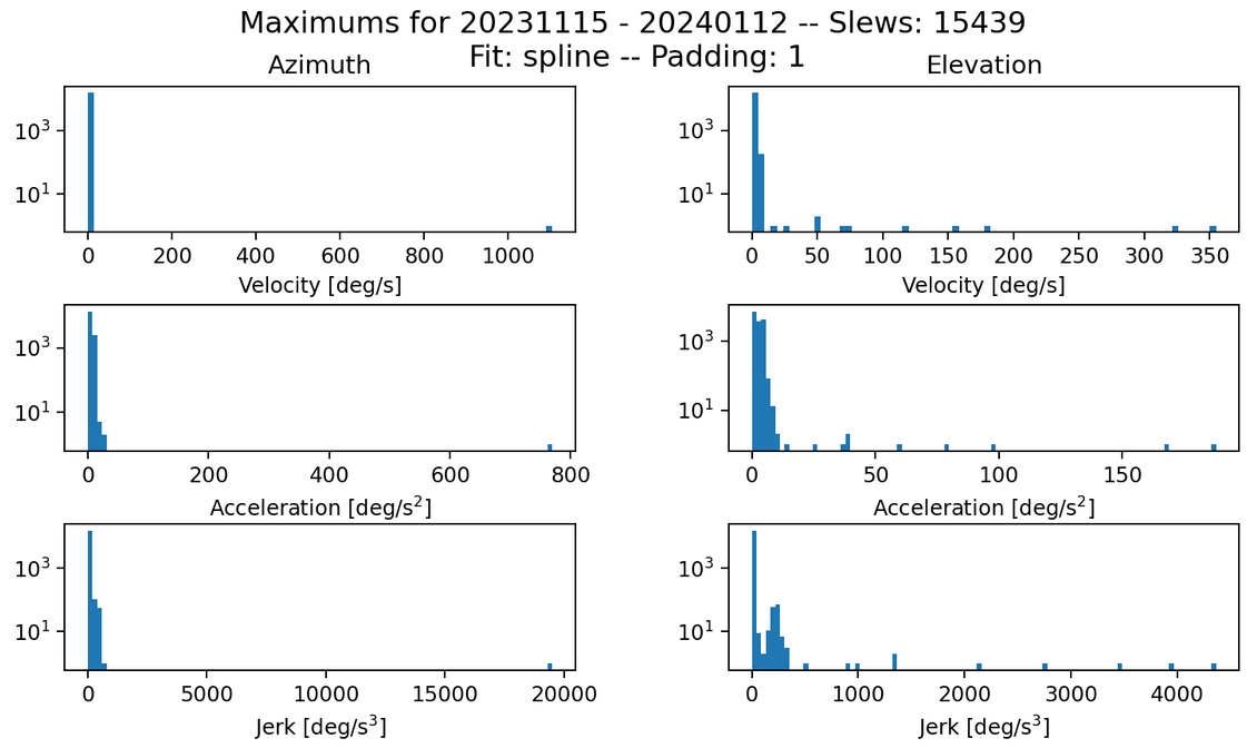
Fig. 1 Max histogram for all slews from November to January. Failures in jerk: 193 azimuth and 198 elevation.#
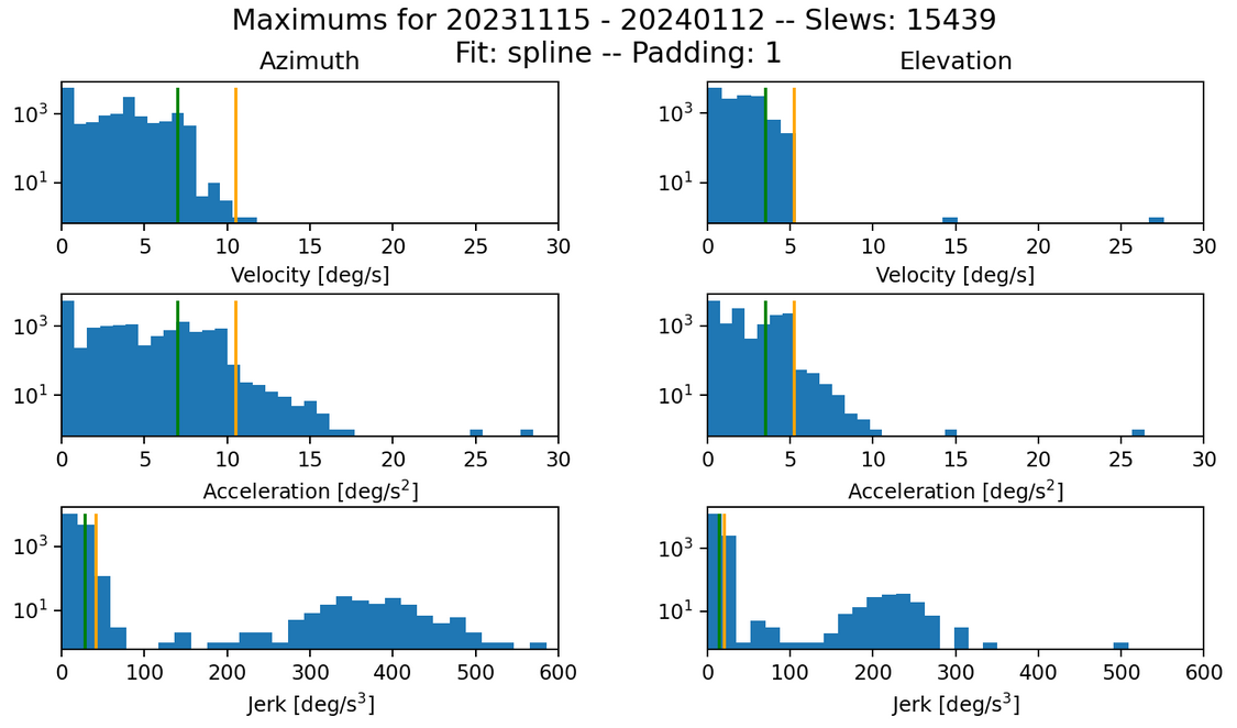
Fig. 2 Same data as figure 1, but zoomed in to show detail without the major outliers.#
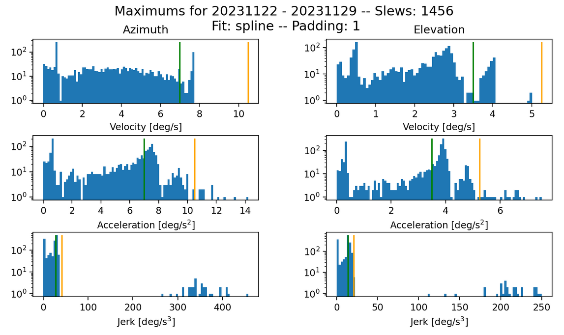
Fig. 3 Max histogram for SOAK Block-137 test slews in November. Failures in jerk: 32 in both azimuth and elevation.#
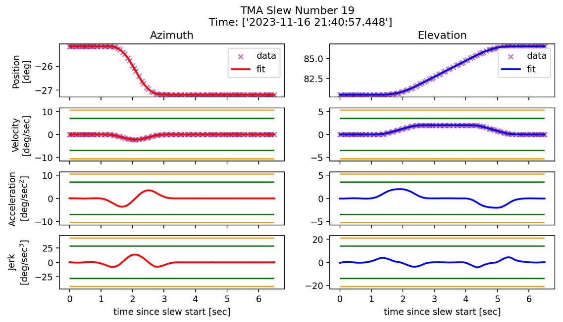
Fig. 4 Slew profile for normal TMA movement.#
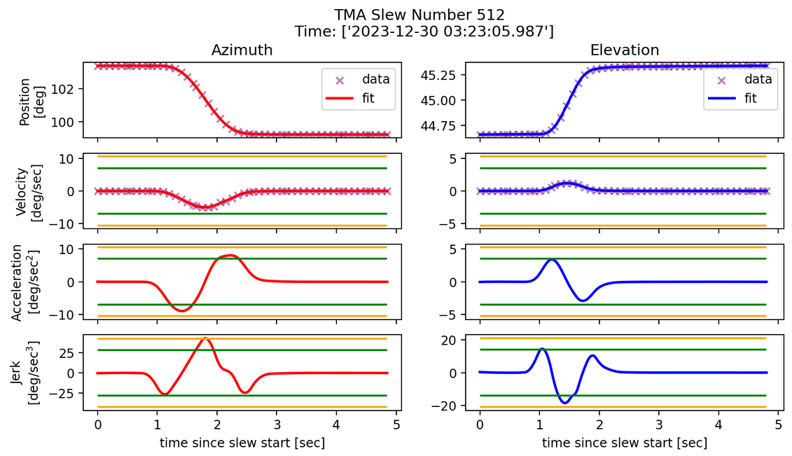
Fig. 5 Typical failed slew profile, failed in azimuth jerk.#
3.2 Improvements from padding#
The first biggest improvement is the addition of padding, where adding 1 second includes both 1 second of data before and 1 second of data after the slew. This addition removes problematic slews caused by sudden starts and stops at the end of slews, which are exacerbated by the double derivative in jerk. The kernel size and smoothing parameter are set to 100 and 0, respectively for this section.
With the SOAK test sample, 134 slews in azimuth and 225 slews in elevation that fail with 0 padding are removed by adding 1 second of padding. Granted, some of these slews may overlap if they fail in both azimuth and elevation. It’s also unclear why the 0 padding setting finds fewer slews.
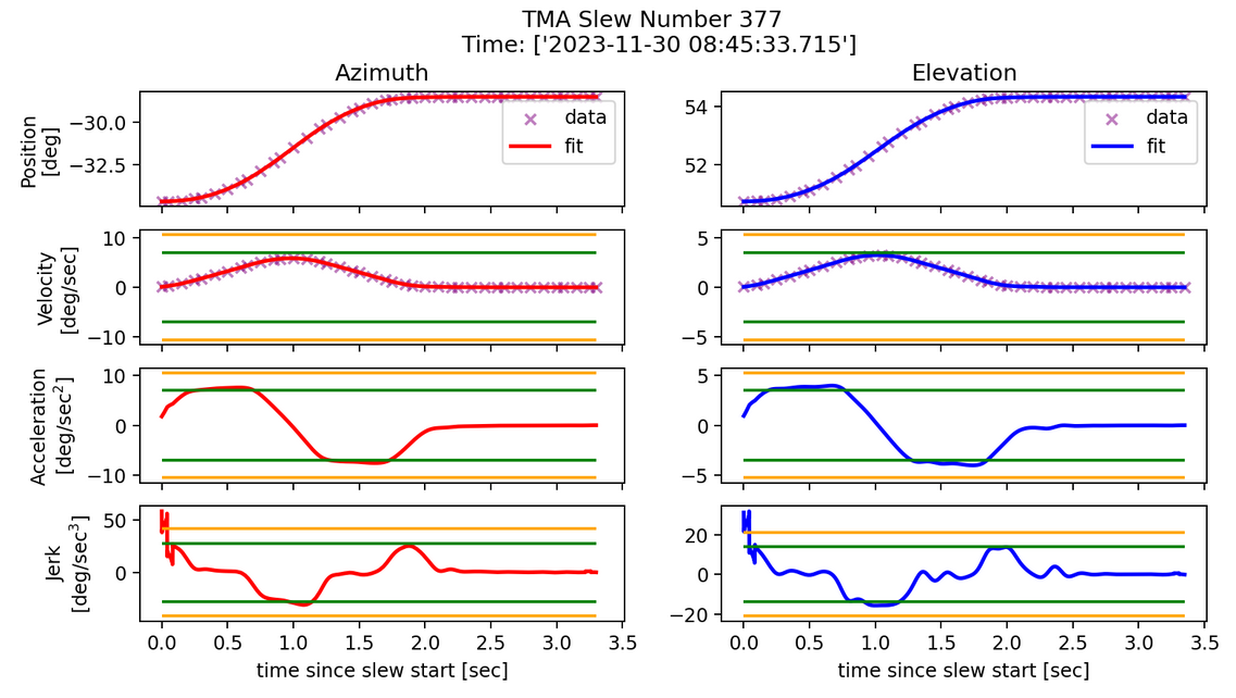
Fig. 6 Failed slew profile where the fit struggles at the ends where movement is occurring. Parameters: s=0 and k=100.#
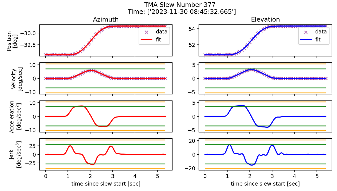
Fig. 7 Same slew as in figure 6 but 1 second of padding is added.#
Padding (sec) |
Total Slews |
# Fails in Azimuth Jerk |
# Fails in Elevation Jerk |
|---|---|---|---|
0.00 |
1388 |
592 |
719 |
0.25 |
1456 |
486 |
495 |
1.00 |
1456 |
458 |
464 |
It’s possible too much padding can detect additional slews that come before or after the actual slew, and produce an artificial edge case, as seen in the slew with 0 padding. However, when this is ran with 0.25 seconds of extra padding, more slews fail.
All other analyses have this 1 second of padding unless stated otherwise.
3.3 Savgol Fit#
The two methods used to fit the data are the spline method and the savgol method. The other parameters used are padding=1 second, smoothing=0, and the kernel size=100.
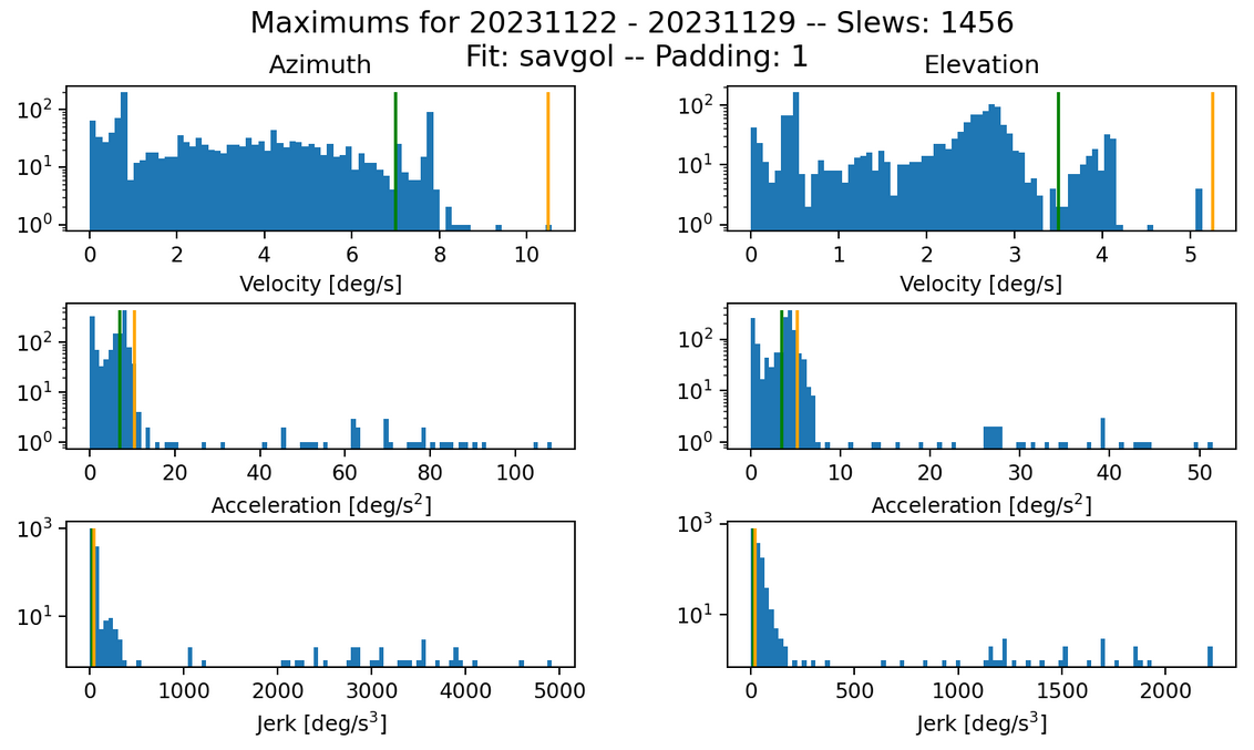
Fig. 8 Max histogram for the savgol fit. Failures in jerk: 559 azimuth and 695 elevation.#
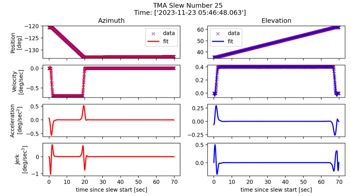
Fig. 9 Example slew profile for savgol fit. Parameters: k=100, s=0.#
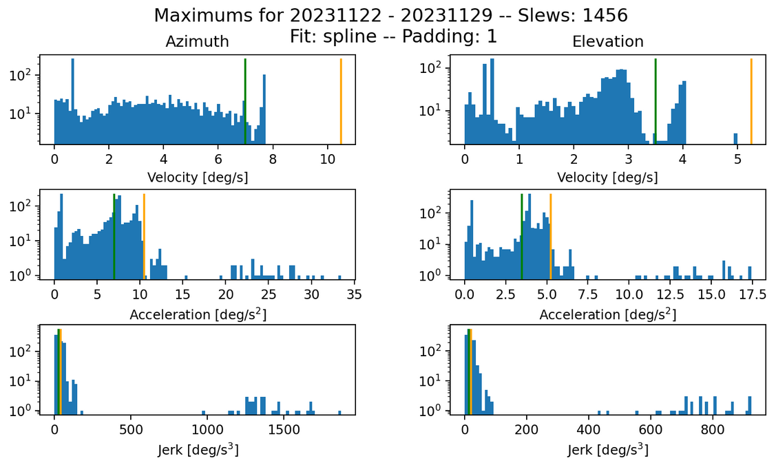
Fig. 10 Max histogram for spline fit. Parameters: k=100, s=0. Failures in jerk: 458 azimuth and 464 elevation.#
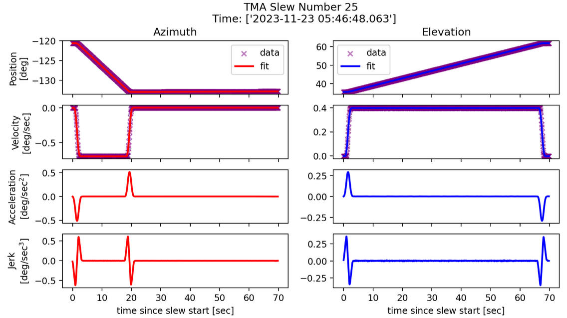
Fig. 11 Slew profile for spline fit. Parameters: k=100, s=0.#
It appears that the spline method tends to work better in terms of fewer failed slews at these parameters, as the spline finds 101 fewer failed slews in azimuth, and 231 fewer in elevation. In the savgol profile plot, it seems that smaller additional peaks are introduced with sudden changes in motion. Given the habit of this analysis exaggerating small changes in velocity into large peaks in jerk, the savgol performance in not surprising. Because of this, the spline method is used for the analysis.
3.4 Parameter Exploration#
Two parameters are explored: the top hat kernel size, k, and the smoothing factor, s. The kernel size essentially acts as the sampling rate, which lower values indicating a higher rate. Too high of sampling can allow outliers in the data to begin affecting the spline, while too low a rate will not fit the data as precisely. The smoothing factor presents a similar scenario where smaller values create a more accurate fit while smaller values offer a smoother fit. The sets of values used for each parameter are {100, 200} and {0.01, 0.1, 0.15, 0.20} for the kernel size and smoothing, respectively. The SOAK test sample with the spline fit using 1 second of padding is used to compare these parameters.
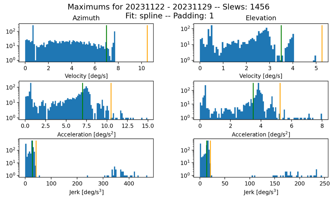
Fig. 12 Max histogram for s=0.01, k=200. Failures in jerk: 34 azimuth and 37 elevation.#
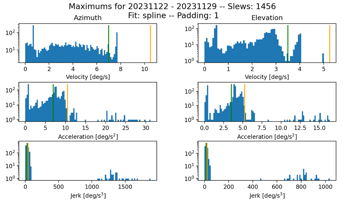
Fig. 13 Max histogram for s=0.10 k=100. Failures in jerk: 393 azimuth and 357 elevation.#
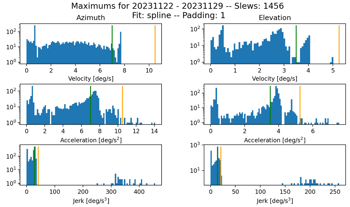
Fig. 14 Max histogram for s=0.10 k=200. Failures in jerk: 32 azimuth and 33 elevation.#
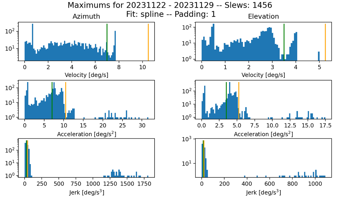
Fig. 15 Max histogram for s=0.15 k=100. Failures in jerk: 373 azimuth and 326 elevation.#
Fig. 16 Max histogram for s=0.15 k=200. Failures in jerk: 32 azimuth and 32 elevation.#
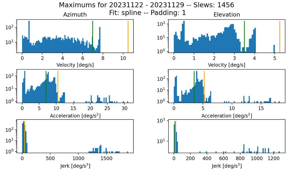
Fig. 17 Max histogram for s=0.20 k=100. Failures in jerk: 359 azimuth and 281 elevation.#
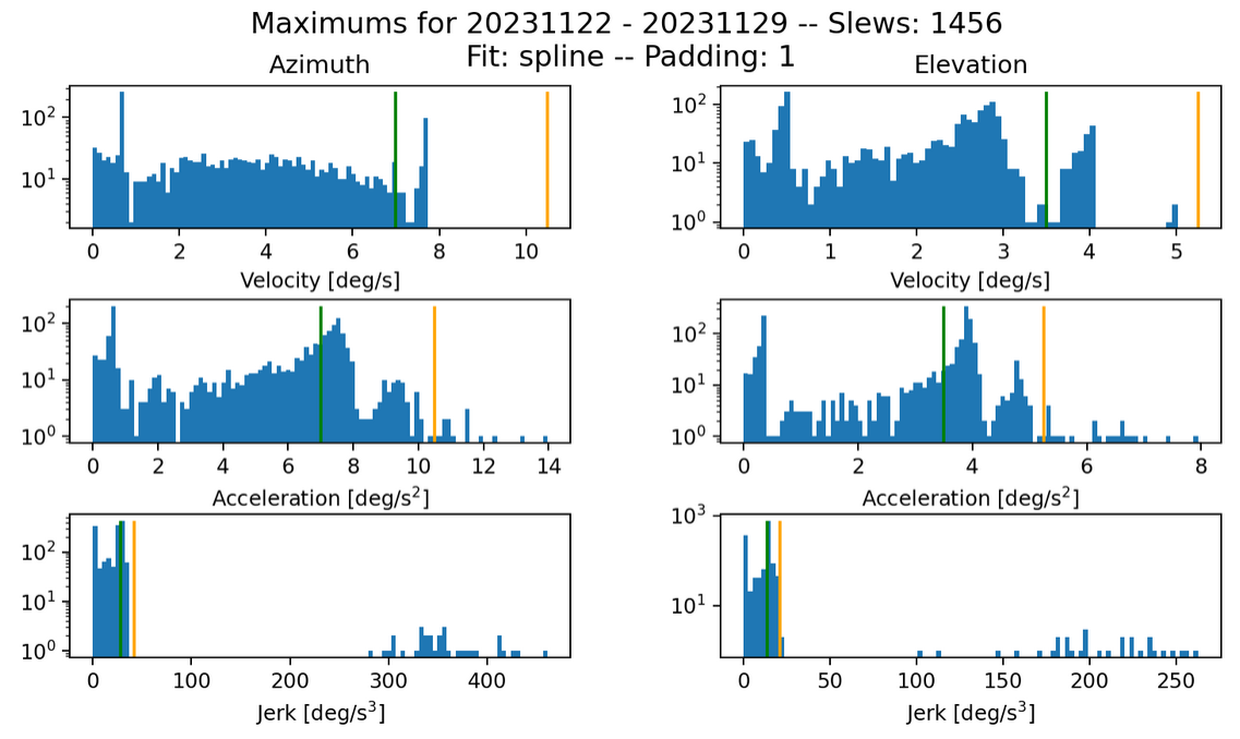
Fig. 18 Max histogram for s=0.20 k=200. Failures in jerk: 32 azimuth and 33 elevation.#
Overall, it seems that the best combination of these two parameters is where k=200 and s=0.15, in terms of the fewest failed slews. The fits seems more sensitive to the kernel size, although increasing the smoothing also improves the number of failed slews. A higher kernel size also decreases the magnitudes of the jerks in failed slews, so while some slews still fail, they fail less drastically.
3.5 Another padding analysis#
As an aside, one more attempt with changing the padding parameter:
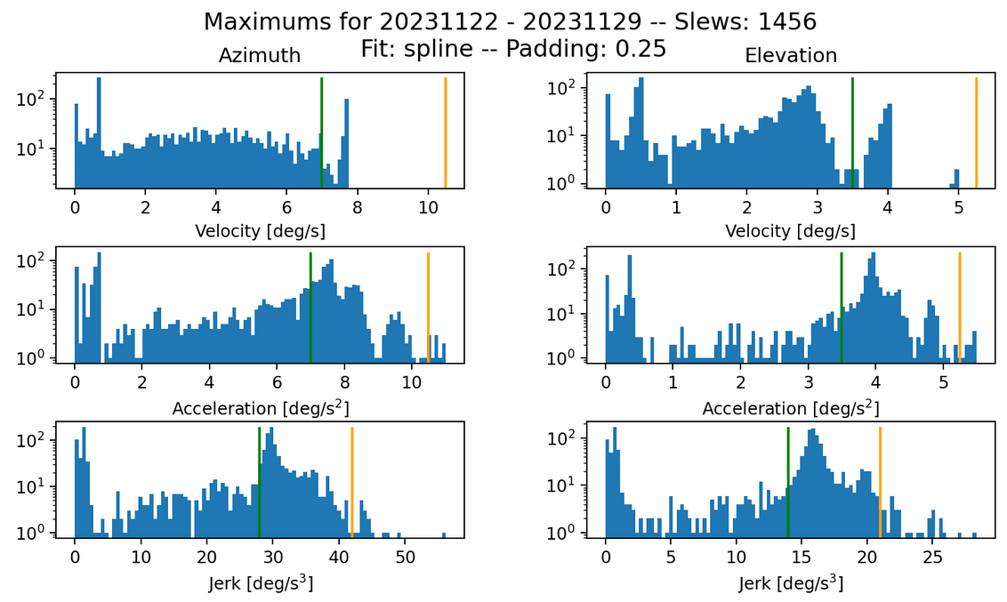
Fig. 19 Max histogram with 0.25 padding s15 and k200. Failures in jerk: 17 azimuth and 32 elevation.#
Given the best kernel size and smoothing parameters found in the other analyses, changing the padding to 0.25 here cuts the number of failed slews in azimuth by almost half. This could provide an explanation of why the 0 padding test found fewer slews; however, in this case the same amount of slews are found while the number of failures still decreases.
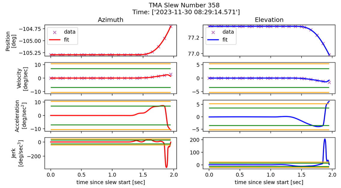
Fig. 20 Slew profile of an offset slew in time. With 1 second of padding on either side, there’s a total of 2 seconds of extra time, which appears to be the whole time in this case. Parameters: k=200, s=0.15.#
4 Summary#
As noted above, this analysis is not enough to accurately determine jerks due to a double derivative from velocity. It’s also difficult to determine whether the slew itself is failing or if the fit is not accurate, given that the number of failed slews have a high sensitivity to both the kernel size and the amount of padding.
For the entirety of the data from 2023/11/15 to 2024/11/13, the parameters deemed best are the following:
A spline fit
1 second of padding
Kernel size of 200
Smoothing factor of 0.15
The number of failed slews for the entire range of data is 193 in azimuth (1.25%) and 198 in elevation (1.28%), and noting that some of these slews may overlap if a slew fails in both azimuth and elevation.
As for the SOAK test sample, the best performance was with the following parameters, where 17 failed in azimuth (1.17%) and 32 in elevation (2.20%).
A spline fit
0.25 seconds of padding
Kernel size of 200
Smoothing factor of 0.15
5 Appendix#
5.1 Previous Work#
5.1.1 Methods
A previous version of this analysis has been done for every slew between 2022/11/01 and 2023/03/30. A cubic spline was used, and the top hat kernel size was set to 100.
Slews were identified using the method found in SITCOMTN-067. The relevant tables were lsst.sal.MTMount.command_trackTarget, lsst.sal.MTMount.logevent_azimuthInPosition, and lsst.sal.MTMount.azimuth/elevation. The beginning of slews were identified with the az_track timestamps, while the ends were defined with 'inPos'==True. With this method applied to all slews, mismatched slews occurred. Another method was to use only the position encoder data, but was less reliable.
To match slew starts and stops, each slew start was matched with the closest slew stop that came after the start. The next slew start was then verified to come after the previous slew stop.
5.1.2 Results
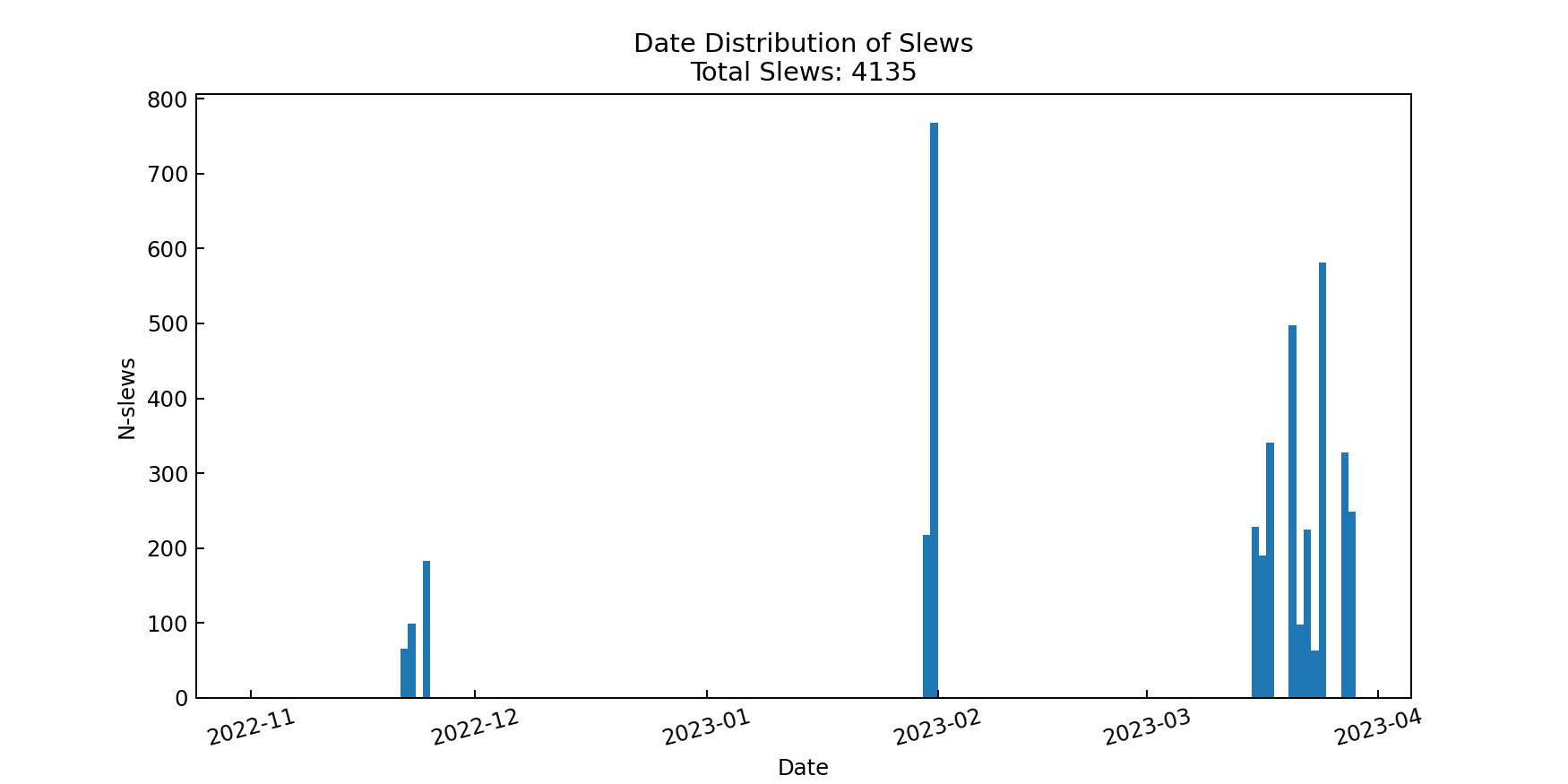
Fig. 21 Data distribution of identified slews.#
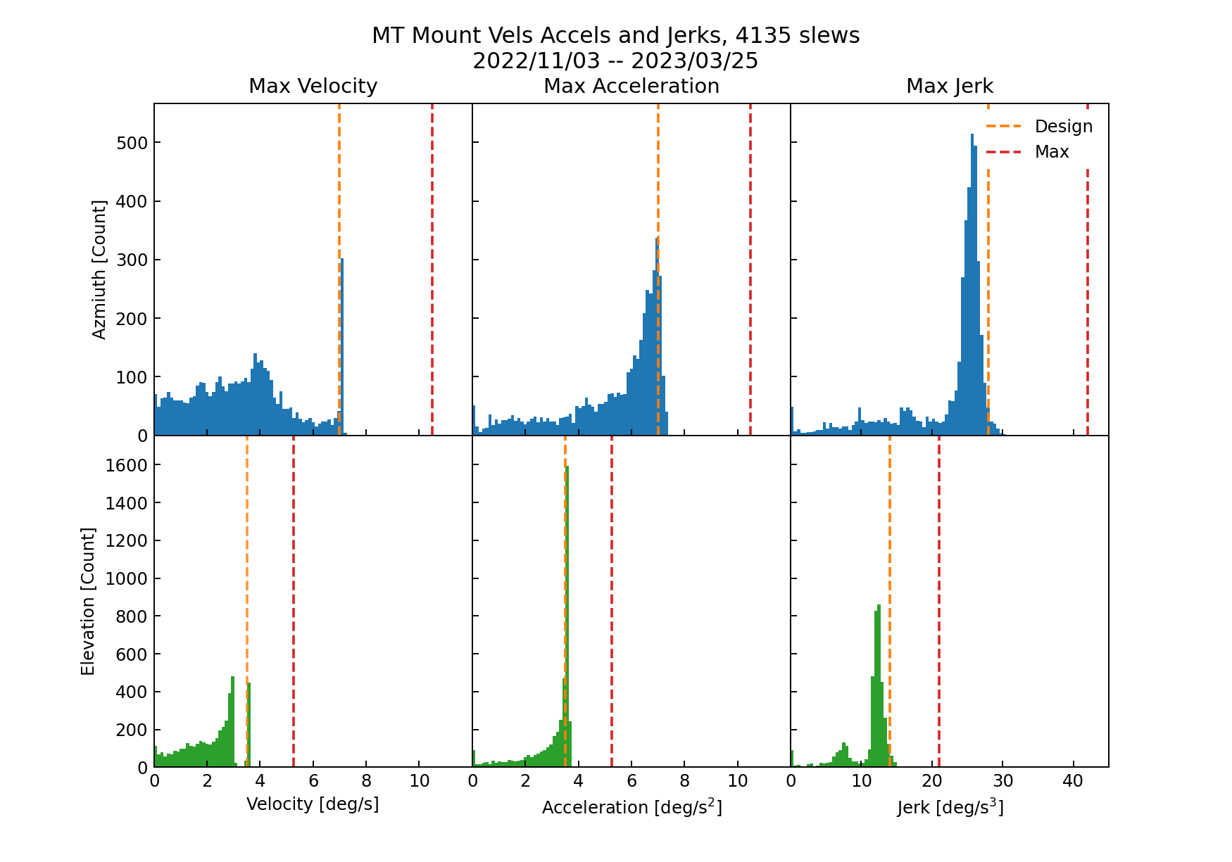
Fig. 22 Distribution of max velocities, accelerations, and jerks for all identified azimuth and elevation slews. Orange indicates design limit, while red is the max limit.#
With this data, 19 slews were flagged for exceeding the maximum limits. An example slew profile plot is shown. Flagged slews had poor fits that could be corrected by hand to keep within telescope specifications.
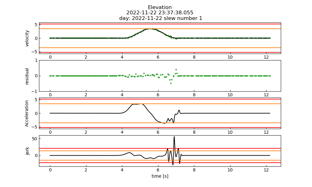
Fig. 23 An example of a slew that was identified as failing the max jerk specification, but as with all flagged slews the failure was an obvious fit failure.#
The included table lists off the start times of all flagged slews with the added 4 second padding beforehand.
Day |
slew start |
|---|---|
2022-11-22 |
01:15:06.047 |
2022-11-22 |
01:17:32.597 |
2022-11-22 |
02:12:41.523 |
2022-11-22 |
02:16:36.322 |
2022-11-22 |
23:37:01.065 |
2022-11-22 |
23:52:13.027 |
2022-11-23 |
00:06:12.465 |
2022-11-23 |
01:06:44.776 |
2022-11-23 |
01:14:20.664 |
2022-11-23 |
01:28:16.824 |
2022-11-23 |
01:29:32.930 |
2022-11-23 |
01:30:10.530 |
2022-11-23 |
01:32:42.886 |
2022-11-25 |
04:57:48.152 |
2022-11-25 |
05:08:37.656 |
2022-11-25 |
08:36:23.112 |
2022-11-25 |
08:37:39.212 |
2022-11-25 |
08:56:41.242 |
2022-11-25 |
08:52:52.826 |